Markov Decision Process

The Markov Decision Process () is the core problem model of reinforcement learning. Whether training a quadruped robot to walk or having a robotic arm complete a grasping task, the first step is always to model the problem as an MDP — specifying the state space, action space, state transition probabilities, and reward function.

Embodied Intelligence Perspective: Taking robotic arm grasping as an example, the state can be joint angles + object pose, the action is the target torque for each joint, and the reward is the signal of whether the grasp succeeded. Once these elements are defined, RL algorithms can be used to find the optimal policy.

Agent-Environment Interaction

As shown in Figure 1, the agent () interacts with the environment () over a series of discrete time steps. At each time step , the agent receives the environment state and selects an action based on that state. After executing the action, the agent receives a reward , and the environment transitions to the next state .

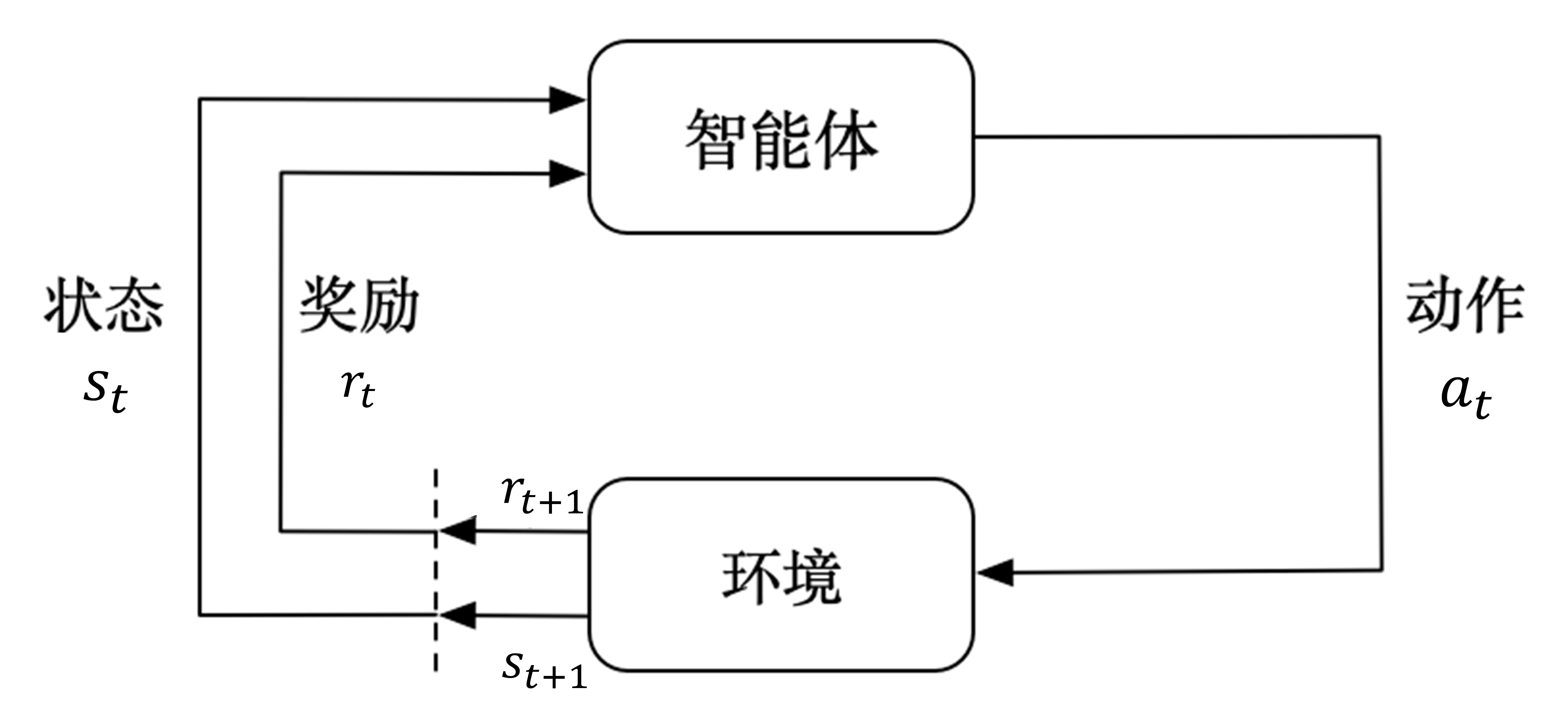
This process repeats continuously, forming a trajectory:

Completing a full trajectory (from initial state to terminal state) is also called an episode (), which typically ends after a finite number of time steps .

To solve a problem with reinforcement learning, the first step is to model it as a Markov Decision Process — specifying the state space, action space, state transition probabilities, and reward function. This is typically defined as a five-tuple:

where is the state space, is the action space, is the state transition probability matrix, is the reward function, and is the discount factor (ranging from to ).

The Markov Property

The core assumption of the Markov Decision Process is the Markov property: the probability distribution of future states depends only on the current state and action, and is independent of past states and actions:

In real robot scenarios, the Markov property is rarely strictly satisfied. For example, in robot navigation, a single lidar scan may not fully describe the environment state (due to occlusion). However, in most cases, the Markov property can be approximately satisfied through appropriate state representations (such as stacking historical frames). Such a process is called a Partially Observable Markov Decision Process (POMDP).

State Transition Matrix

For finite state spaces, a state flow diagram can represent transition relationships between states. As shown in Figure 2:

The transition probabilities between states can be represented as a matrix:

where is the number of states. The transition probabilities from any given state to all other states sum to . The state transition matrix is part of the environment, describing the transition relationships between environment states.

Objective and Return

The agent's objective is to learn an optimal policy through interaction with the environment, such that the actions chosen in each state maximize the cumulative reward. This cumulative reward is called the return:

The discount factor controls the importance of future rewards in current decision-making. When is close to , the agent focuses more on immediate rewards; when is close to , it places greater emphasis on future rewards.

The discount factor can be used to measure the agent's concern for long-term returns, known as the effective horizon:

When , , meaning the agent considers rewards within the next time steps. In robot walking tasks, a large is typically needed to account for long-term locomotion stability.

Recursive definition of the return:

Policy and Value

Policy

A policy () represents the rule by which an agent selects actions in each state, denoted by :

A policy can be deterministic (always selecting the same action in a given state) or stochastic (selecting actions according to a probability distribution). In embodied intelligence, stochastic policies are more commonly used because they provide better exploration capability and robustness.

State Value

The state value function represents the expected return when starting from a given state and following policy :

Action Value

The action value function represents the expected return given a state and action :

Relationship Between State Value and Action Value

The state value is the weighted average over all possible action values. The state value reflects the quality of the policy itself, while the action value more specifically reflects the quality of choosing a particular action in a given state.

Model-Based vs Model-Free

• Model-Based methods: Use the environment model (state transition probabilities and reward function) for planning and decision-making, such as dynamic programming. In simulation environments, the environment model can sometimes be obtained to accelerate learning.
• Model-Free methods: Do not rely on the environment model, learning through direct interaction with the environment, such as PPO and SAC. These are more widely applied in real robot scenarios, since accurate dynamics models of real environments are typically difficult to obtain.

Prediction and Control

• Prediction: Evaluate the quality of a given policy, i.e., compute the value function.
• Control: Find the optimal policy that maximizes cumulative return.

In complex problems, prediction and control typically need to be solved simultaneously — learning the optimal policy while evaluating the current policy's quality (this is precisely the idea behind the Actor-Critic framework).